Matrix maths for quantum physics

Reading David Deutsch’s papers on quantum physics requires knowing some matrix maths. The papers are here

https://arxiv.org/abs/quant-ph/9906007

https://arxiv.org/abs/quant-ph/0104033

https://arxiv.org/abs/1109.6223

This post gives a brief account of the relevant maths.

Complex numbers

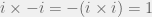
First, a brief explanation of complex numbers. Ordinary positive and negative numbers have the property that the square of the number is positive, e.g. 1\times 1=1,5\times 5=25,-12\times -12=144. An imaginary number is defined to have the property that its square is negative. The imaginary number i is the number such that i\times i=-1 and other imaginary numbers are just multiples of i. Also, i\times -i = - (i\times i)=1A complex number is a sum of an ordinary real number and an imaginary number, e.g. 1+2i is a complex number.

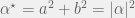
For a complex number \alpha given by a +bi the complex conjugate\alpha^\star of\alpha is defined as a -bi. Now, \alpha \time\alpha^\star =a^2 +b^2 =  |\alpha|^2 and  |\alpha| is called the magnitude of \alpha. For a real number  \theta(\cos\theta)^2+(\sin\theta)^2 = 1, so for any complex number, there is a real number \theta such that \alpha= |\alpha|(cos\theta+\sin\theta i). It also happens to be true that e^{i\theta} = cos\theta+\sin\theta i and so a complex number\alpha is sometimes represented as |\alpha|e^{i\theta}

Matrices

These papers are about the multiverse as described by quantum mechanics. Each system exists in multiple versions that can interact in interference experiments. For any particular quantity you could measure for which there are multiple possible outcomes, there is one version of the system for each outcome. There is a finite set of possible measurement results for any finite system.

Let’s suppose that we have a system S and a measurement that could be performed on S with two possible outcomes +1,-1. There needs to be something in the theory that represents the transitions between each outcome. There is a complex number n_t that describes each transition t: the probability of the transition is |n_t|^2. So for S the thing that represents these transitions would need 4 numbers: one for each pairs of outcomes(+1,+1),(-1,-1),(+1,-1),(-1,+1). Now, a version of the system could do the transition (+1,-1) and then it could do any of the transitions allowed from -1. The system could also do any -1 transition if it did the transition (-1,-1).

What happens if two transitions happen one after another? The way to work out what happens is you list the set of possible states of the system. You can describe the first set of transitions as a square matrix whose elements are the numbers for each transition. So for the system S the matrix would read:

\begin{bmatrix}n_{(-1,-1)} & n_{(-1,+1)}\\  n_{(+1,-1)} & n_{(+1,+1)}\end{bmatrix}

The second transition would have a different set of numbers m_t and the corresponding matrix would be:

\begin{bmatrix}m_{(-1,-1)} & m_{(-1,+1)}\\  m_{(+1,-1)} & m_{(+1,+1)}\end{bmatrix}

To work out the number for the composition of the transitions, you take the product of the transitions for which the final state of the first transition is the same as the initial state of the next transition and add them together. The matrix that describes the result of both transitions would be:

\begin{bmatrix}m_{(-1,-1)}n_{(-1,-1)}+m_{(-1,+1)}n_{(+1,-1)} & m_{(-1,-1)}n_{(-1,+1)}+m_{(-1,+1)}n_{(+1,+1)} \\  m_{(+1,-1)}n_{(-1,-1)}+m_{(+1,+1)}n_{(+1,-1)} & m_{(+1,-1)}n_{(-1,+1)}+m_{(+1,+1)}n_{(+1,+1)} & \end{bmatrix}

This is just the equation for the result of multiplying a pair of 2\times 2 matrices. More generally, for a set of N possible states a set of transitions is represented by an N\times N matrix. If two sets of transitions are represented by matrices A and B, the transition that happens if you do the transition described by A followed by the transition described by B is described by the matrix product of B and A, whose elements are (BA)_{ij}=\sum_kB_{ik}A_{kj}. For more than two transitions you just multiply more matrices, with the earlier transitions on the right and the later ones on the left.

So far I have only described transitions. What describes the system undergoing the transitions? The answer is more matrices. You need a set of matrices that can be multiplied by complex numbers and added up to give any other matrix of the same dimension. The reason is that you need a set of matrices that can be used to represent all of the possible transitions. For a system with N possible states you need N^2 matrices. If A is a transition matrix and M is one of the matrices describing the system then the system after the transition is described by A^\dagger M A, where A^\dagger is the Hermitian conjugate of A: the matrix found by taking the complex conjugate of the entries and interchanging their indices. So the Hermitian conjugate of

\begin{bmatrix}a & b\\  c & d\end{bmatrix}

is given by

\begin{bmatrix}a^\star & c^\star \\  b^\star  & d^\star \end{bmatrix}

The matrices representing the transitions are unitary, which means that A^\dagger A = I where is the identity matrix that has 1s on the diagonal and zero on all off-diagonal entries. Some examples of unitary matrices:

\begin{bmatrix}1/\sqrt{2} &1/\sqrt{2} \\  1/\sqrt{2} & -1/\sqrt{2} \end{bmatrix}

\begin{bmatrix}1 &0 \\  0 & i \end{bmatrix}

Measurable quantities are represented by eigenvalues (the definition will given below, but requires some setup) of Hermitian matrices. A Hermitian matrix M is a matrix for which M^\dagger = M. Some examples of Hermitian matrices:

\sigma_3 = \begin{bmatrix}1 & 0 \\  0 & -1 \end{bmatrix}

\sigma_2 = \begin{bmatrix}0 & -i \\  i & 0 \end{bmatrix}

\sigma_1 = \begin{bmatrix}0 & 1 \\  1 & 0 \end{bmatrix}

\sigma_0 = I = \begin{bmatrix}1 & 0 \\  0 & 1 \end{bmatrix}


These matrices are called the Pauli matrices. Suppose a matrix M and a vector v have the property Mv = av, where a is a number, then a is an eigenvalue of M and is an eigenvector of M. The first three Pauli matrices \sigma_1,\sigma_2,\sigma_3  all have eigenvalues +1 and -1. The eigenvectors for \sigma_3 are $latex[1,0],[0,1]$. The eigenvectors for \sigma_2 are 1/\sqrt{2}[1,1],1/\sqrt{2}[1,-1]. The dot product of two vectors v = (v_1,v_2\dots),w = (w_1,w_2\dots) is given by v\dot w =v_1w_1+v_2w_2+\dots. The dot product of two eigenvectors is always zero: they are said to be orthogonal.


A projector P is an operator such that  P^2=P. The projectorsI+\sigma_j,I-\sigma_j for the three Pauli matrices \sigma_1,\sigma_2,\sigma_3 have the property that \sigma_j P = P or\sigma_j P = -P . More generally, for any Hermitian matrix M there is a set of projectors P_j such that P_jP_k = \delta_{jk}P_j where \delta_{jk} = 1 if j=k and 0 otherwise for which M = \sum_j a_jP_j and the a_j numbers are the eigenvalues of M.

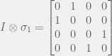
If you have two different systems S_1,S_2, the transition matrices and the matrices representing the system’s state can be represented by tensor products of the matrices representing each system. The tensor product of two matrices A,B is denoted as $latex A\otimes B$ and is represented by

\begin{bmatrix}a_{11}B &a_{12}B &\dots \\  a_{21}B &a_{22}B&\dots\\  \vdots& \vdots & \ddots \end{bmatrix}

For example

I\otimes \sigma_1 =\begin{bmatrix}  0 & 1 & 0 & 0\\  1 & 0 & 0 & 0\\  0 & 0 & 0 & 1\\  0 & 0 & 1 & 0  \end{bmatrix}

A function f applied to a Hermitian operator M = \sum_j a_jP_j is given byM = \sum_j f(a_j)P_j.

I think that covers most the matrix stuff you need to know to read those papers. More stuff on matrices can be found in Quantum Computation and Quantum Information by Nielsen and Chuang, which also has exercises.

About conjecturesandrefutations
My name is Alan Forrester. I am interested in science and philosophy: especially David Deutsch, Ayn Rand, Karl Popper and William Godwin.

Leave a Reply

Fill in your details below or click an icon to log in:

WordPress.com Logo

You are commenting using your WordPress.com account. Log Out /  Change )

Facebook photo

You are commenting using your Facebook account. Log Out /  Change )

Connecting to %s

%d bloggers like this: